[adsense:responsibe:9545213979]

Problemas, examenes, practicas y simulaciones de: Regulacion(Scilab), Electronica(Micro-Cap; Spice) y Estadistica (R-Projec..
Problema 1 (Bode, error de posicion, compensador de atraso)
Solapas principales
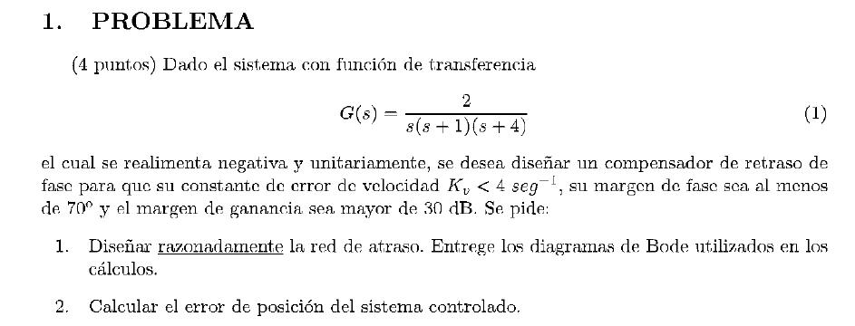
SOLUCION:
Apartado 1 (Diseñar razonadamente la red de atraso)
-
Primeramente vamos a calcular la K dada por el error de velocidad

 Con lo que el sistema G1(s) nos queda:
-
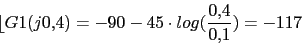
Vamos a calcular la nueva frecuencia de cruce wc, sabiendo el margen de fase necesario
w 0.1 0.4 1 4 10 40 
-90 (0) -90 (0) -90 (0) -90 (0) -90 (0) -90 
0 (-45) (-45) -45 (-45) (-45) -90 (0) -90 
0 (0) 0 (-45) (-45) -45 (-45) (-45) -90 -90 (-45) -117 (-90) -152.81 (-90) (-90) (-45) -270 El valor de wc viene dado por la frecuencia que tiene el siguiente angulo de fase:
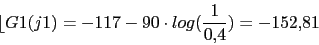
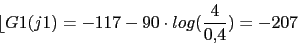
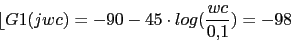
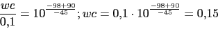 Esta sera la nueva frecuencia de corte
 -
Vamos a escoger
 tal que
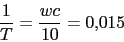
4. Vamos a calcular ![]()
![]()
![]()
| w | 1 | 4 | |||
|
|
(-20) | (-20) | (-20) | ||
|
|
(0) | (-20) | (-20) | ||
|
|
(0) | (0) | (-20) | ||
| (-20) | 12.04 | (-40) | -12.04 | (-60) |
![]()
![]()
![]()
![]()
Con lo que ya tenemos casi el compensador:
5. Ahora vamos a calcular la ![]()
![]()
![]()
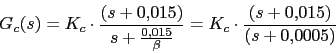
Con lo que el compensador nos queda:
![]()
La fase en wc del sistema es:
![]()
Con lo que el margen de fase como vemos a continuacion verifica las condiciones
Vamos a calcular el margen de ganancia
| w | 5E-5 | 5E-4 | 1.5E-3 | 5E-3 | 1.5E-2 | 1.5E-1 | |||||
|
|
0 | (-45) | -45 | (-45) | (-45) | -90 | (0) | -90 | (0) | -90 | |
|
|
0 | (0) | 0 | (0) | 0 | (45) | (45) | 45 | (45) | 90 | |
| G1(s) | 0 | (-45) | -45 | (-45) | (0) | (45) | -45 | (45) | 0 | ||
| -90 | (0) | -90 | (0) | -90 | (0) | -90 | (0) | -90 | () |
![]()
![]()
![]()
Verifica las condiciones de margen de ganancia
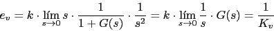
Apartado 2 (Vamos a calcular el error de posicion del sistema controlado)
![]()
Como el sistema es de tipo I. El error de posicion va a ser cero.
![]()
![]()
![]()
Vamos a hacer los calculos y las comprobaciones de resultados con el Scilab
clear;
s=%s;
g=2/(s*(s+1)*(s+4));
gs=syslin('c',g);
aux=horner(s*gs,0)
kv=4;
k=kv/aux
g1=k*gs
fwc=-180+70+12
wc=0.1*10^((fwc+90)/(-45))
aux2=horner(g1,%i*wc)
aux3=atan(imag(aux2),real(aux2));
aux4=360*aux3/(2*%pi)
a=wc/10;
aux5=20*log10(abs(aux2))
g1015=20*log10(4)-20*log10(0.15)
g04=20*log10(4)-40*log10(4)
bet=10^(g1015/20)
b=a/bet
kc=k/bet
gc=kc*(s+a)/(s+b)
gt=g*gc;
gts=syslin('c',gt);
aux6=horner(gts,%i*5)
aux7=20*log10(abs(aux6))
s1=s/(2*%pi)
gb=2/((s1+0.000000001)*(s1+1)*(s1+4));
gcb=kc*(s1+a)/(s1+b);
gtb=gb*gcb;
gbs=syslin('c',gb);
gcbs=syslin('c',gcb)
gtbs=syslin('c',gtb)
[mg,frg]=g_margin(gtbs)
[mp,frp]=p_margin(gtbs)
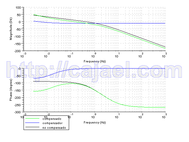
clf;
bode([gbs;gcbs;gtbs],['compensado';'compensador';'no compensado'])
Español


Búsqueda personalizada
Idiomas
 English
 Español
Comentarios recientes
- Muy bueno hace 10 años 3 meses
- good hace 10 años 3 meses
- Engranajes hace 10 años 3 meses
- REVISAR hace 10 años 4 meses
- UTIL hace 10 años 4 meses
- Realimentación hace 10 años 7 meses
- Hello There. I found your hace 10 años 7 meses
- Good web site! I really love hace 10 años 7 meses
- Well I really enjoyed reading hace 10 años 7 meses
- Thanks again for the blog hace 10 años 7 meses
Seguidores en Google
Busquedas populares
Inicio de sesión
Contenido popular
- 6 Problema 1 (Diodos, resistencia dinamica, Shockley)
- Ejercicion 4 (Estabilidad, Criterio de Routh)
- Examenes 2009 RI
- 3.1.2 Calculo de los parámetros híbridos con Micro-Cap
- Problema 1 (Bode, compensador de adelanto, error de velocidad, margen de fase y margen de ganancia)
- SISTEMAS MECANICOS
- Apartada c) del Ejercicio 2 Campos y Ondas 1402S2 (Potencia onda incidente; Potencia onda reflejada; Potencia onda transmitida)
- 1.4.2 Montaje practico del circuito RC en serie
- 1.3 Simulación de un circuito RC en serie
- 2.1.1 Calculo teórico del rectificador de onda completa
- Catalogo de baterias industriales de EXIDE (Ingles)
- 2.1 Calculo teórico y simulación del circuito RC con potenciometro
- Ejemplo 9.2 pag633 OGATA
- 2.4 Medir la intensidad con el osciloscopio en el circuito RC con potenciometro
- Cuestion 2 EDiferenciales 1406S2 (Ecuacion diferencial lineal de coeficientes constantes)
- REGULACION AUTOMATICA
- Problema 1 (Bode, regulador, error de posicion)
- Tranformada de Laplace
- Cuestion 1 EDiferenciales 1109S2
- Cuestion 2 EDiferenciales 1206S1
- SIMULACIONES CON SCILAB
- 1.1.2 Simulación con Micro-Cap del rectificador de media onda
- Apartada 1) del Ejercicio 2 Campos y Ondas 1402S1 (Constantes linea de transmision; Constante de propagacion)
- Simulacion estadistica del Ejercicio 6.8 (Distribucion de Poisson)
- Problema B2.1 pag51 OGATA 4ed(Tranformada de Laplace)
Páginas
Today's popular content
- REGULACION AUTOMATICA
- SIMULACIONES CON SCILAB
- Tranformada de Laplace
- Ejemplo 2.6 pag37 OGATA 4edicion(Tranformada de Laplace)
- Ejemplo 2.7a pag38 OGATA 4edicion(Tranformada de Laplace)
- Ejemplo 2.7b pag39 OGATA 4edicion(Tranformada de Laplace)
- Ejemplo 2.10 pag46 OGATA 4ed(Tranformada de Laplace)
- Problema A2.15 pag48 OGATA 4ed(Tranformada de Laplace)
- Problema A2.16 pag49 OGATA 4ed(Tranformada de Laplace)
- Ejemplo 2.17 pag50 OGATA 4ed(Tranformada de Laplace)
- Problema B2.1 pag51 OGATA 4ed(Tranformada de Laplace)
- Problema B2.2 pag51 OGATA 4ed(Tranformada de Laplace)
- Problema B2.3 pag51 OGATA 4ed(Tranformada de Laplace)
- Lugar de las Raices
- Programa 6.1 OGATA 4edicion pag360 (Lugar de las Raices)
- Programa 6.2 OGATA 4edicion pag361 (Lugar de las Raices)
- Programa 6.3 OGATA 4edicion pag362 (Lugar de las Raices)
- Programa 6.5 OGATA 4edicion pag366 (Lugar de las Raices)
- Programa 6.6 OGATA 4edicion pag367
- Programa 6.7 OGATA 4edicion pag367
- Programa 6.8 OGATA 4edicion pag370
- Programa 6.9 OGATA 4edicion pag372
- Programa 6.10 OGATA 4edicion pag378
- Problema A6.11 OGATA 4edicion pag400
- Problema A6.12 OGATA 4edicion pag402
Páginas

Añadir nuevo comentario